Understanding the RF power in a coaxial cable assembly

PublishTime： 2023-10-02 Article Source：Smiths Interconnect Blogs

One of the most often asked questions from our customers about our cable assemblies is “How much power can this cable assembly handle”. My response is usually the same, “It depends”. This question cannot be understood in its completeness without the understanding of power, and the many variables that contribute to the makeup of power transmission. This white paper will serve to shed some light on this issue, and at the same time, give some practical examples seen in the industry. In addition, hopefully, it will explain why it is difficult to just give a chart or table for all of our cable assemblies with regard to power handling.

Why do we need RF Power transmission? In Radar, for example, we transmit high power in order for the signal to be sent at a great distance. Any cable attached to this antenna must be able to handle the same power and thus must be carefully chosen.

Power fundamentally is Energy transferred per unit of Time. A Power amplifier sending energy down a transmission line “transfers” this energy from point A, to point B. You will find a couple of different ways to express power such as “Watts” or “Milliwatts” (mW), as seen in the power amplifier world, or it can be expressed in dBm, (decibels per milliwatt), as we see in the Telecom world.

The basic conversions from one to the other can be seen below:

dBm = 10 Log10 P (milliwatts)

P (milliwatts) = 10 (dBm/10)

For example, the +43dBm signal would be then equal to 19,952 milliwatts or about 20 watts. And a VNA output power of 100 mW is about 20 dBm.

Operating power is important, however, there are other factors needed to determine what cable assembly will fit a certain application. Before discussing this, we need to first look at another important factor of power, and that is Peak Power vs. Average Power.

Peak Power can be defined as that power where what is called the “Voltage Gradient” is at its maximum. In other words, we have in the coaxial cable a potential between the inner conductor and outer conductor. When this potential becomes too large, the voltage will want to jump from the inner to the outer conductor bypassing the insulator medium (Air or PTFE, or other insulation materials). When this “jump” in voltage happens, the voltage gradient is at its maximum. So then Peak Power in a cable assembly is limited by the Voltage Gradient. This is the reason we must pay attention to the “Operating Voltage” of an assembly. The operating voltage is normally set in order not to exceed this voltage gradient. This is one of the main reasons we perform Dielectric Withstanding Voltage (DWV) tests on our assemblies which essentially verify if this voltage gradient is exceeded. Steps need to be taken in connector design, as well as the connector to the cable assembly process, to ensure success.

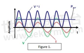
Next, we have Average Power. Once we get passed the limit of Peak Power due to the voltage gradient, we turn to Average Power and concern for dissipating heat. Most of our RF signals are either sinusoidal or pulsed in nature. Figure 1. is an example of a sinusoidal power wave. Average power, also known as Continuous Wave or “CW” power, is what we base most of our calculations on when answering application questions on power handling. Even when the signal is a pulsed square wave as we find in radar applications, this can be reduced to average power by multiplying the Peak power by the duty cycle. For example, a 500 W peak signal with a 10% duty cycle, equates to a 50W average power signal.

So, what are these variables that affect power in our cables as mentioned earlier? The first one is Frequency. The main premise being as the frequency increases, the power decreases. The simple reason is that due to the laws of Microwave Signal Transmission, higher frequencies are supported and transmitted in smaller cables, and the smaller the cable, the harder to dissipate the heat resulting in power loss.

The second variable is VSWR. Reflections caused by mismatches in impedance will also account for power losses in a cable assembly. At any point on a transmission line where the impedance doesn’t match the characteristic impedance, you will have a mismatch, and therefore VSWR (or Return Loss). Since part of the power signal was “returned”, we have power loss.

The third variable is Altitude. Normally when power figures are given for a particular assembly, you might see a qualifier such as “Sea Level”. The reason is that power for a cable is different at Sea Level than say at 70k ft. So, we need to derate a cable for altitude. The reason is due to the air molecules. Air molecules are excellent in removing heat away from hot objects. The higher in altitude, the less air molecules, so we need to account for this in our power ratings. The below chart in Figure 2. displays the derating factor at different altitudes. Simply put, if you have a cable that can handle 50 watts at Sea Level, then that same cable can only handle 14.5 watts at 70,000 feet.

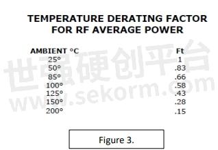
The final variable in the Power transmission equation is Temperature. This was alluded to before regarding cable size and the ability to dissipate heat. However, we also have the environment around the assembly to consider, and this will affect the performance of power. The high current in the center conductors increases the temperature rather quickly. Copper is a common conductor material, great for conducting electrical signals as we as heat. This heat needs to dissipate from the assembly to maintain its current power level. If the environment outside the assembly is at a high temperature, then this dissipation is slower or not possible at all. Because of this, we need also to derate an assembly with respect to temperature (see Figure 3.).

How then do we calculate the power handling capability of our cable assemblies? First, we need to know the power requirement (average or CW), frequency, temperature, and altitude of the application. Next, the connectors need to be identified. With this information, an average power figure can be calculated.

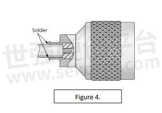
We need to understand that the cable assembly is made up of cables and connectors. The power possible in the assembly is dependent on both the cable and connectors, and either can be the weakest link. It is also worth noting that the cable/connector junction can often be the point of lowest power transmission (see Figure 4.).

The two examples below will illustrate the issue of connector vs. cable. The first example is a Type N connector mounted on a .047 s/r cable operating at 6 GHz. In this example, the connector can handle about 1200 W at sea level and 25 deg C. The cable on the other hand, can only handle about 21 W. So, a cable assembly with this criterion must start at 21 watts when considering power. The second example is an SMA connector mounted on our Lab-Flex 290 cable. At the same frequency of 6 GHz, the power capability of the SMA is about 150 watts, with the power capability of the 290 cable at about 1800 watts. Therefore, we can’t just look at the power capability of the cable, as it might not be the weakest part of the equation. These two examples are the two extremes of what can happen. Keep in mind as mentioned before that the cable/connector junction in Figure 4. may also be the weakest link. In addition, if the assembly is to be used at a higher altitude or temperature, it needs to be derated as noted above.

One final thought about connector interfaces, and how they relate to power. There are some connectors that can reach a higher power rating than others. This has to do with the construction of the interface. Remember the discussion above regarding the voltage gradient. Interfaces typically are designed with PTFE or Air or a combination of the two. These materials will dictate how much power the interface can handle. This voltage gradient is related to the “dielectric strength” of a material. It so happens that the dielectric strength of air is 70 volts/mil, and for PTFE it's 1000 volts/mil. This means that for an air interface, every .001” gap between two metal surfaces, you can have a potential of 70 volts, above which you will reach a maximum voltage gradient. PTFE has a dielectric strength of much greater magnitude. This is generally why a standard TNC interface can handle much more power than an SMA interface. See Figure 5. & Figure 6.

You can see by the two interfaces above that there is a much shorter path from the center conductor to the outer conductor in the SMA design, than in the TNC design. In addition, the TNC design has insulators that fit one inside the other. This increases the conductive path from the center conductor to the outer conductor and therefore increases the power capability.

So, in summary, the power capability of a coaxial cable assembly is dependent on the voltage gradient throughout the assembly. The average power of an assembly can be computed readily if the frequency, altitude, and temperature are known, and the VSWR is approximated. We must understand the power capabilities of both the connectors and the cable to get the full picture. Lastly, interface design is key to higher power operation with PTFE being a better interface material especially if it’s a telescoping type design seen in Figure 5.

The above information should shed some light on the difficulty of just displaying a chart or graph of all the different power possibilities for our cables. If such power information is needed, please forward the details of your application to us, and we will be quick to respond with your information.

+1 Like
Add to Favorites

Recommend

Technical Resources

More>

New Products & Solutions

More>

This document is provided by Sekorm Platform for VIP exclusive service. The copyright is owned by Sekorm. Without authorization, any medias, websites or individual are not allowed to reprint. When authorizing the reprint, the link of www.sekorm.com must be indicated.

Integrated Circuits